Getting Started

This notebook gets you started with a brief nDCG evaluation with LensKit for Python.

Setup

We first import the LensKit components we need:

from lenskit import batch, topn, util
from lenskit import crossfold as xf
from lenskit.algorithms import als, item_knn as knn
from lenskit.metrics import topn as tnmetrics

And Pandas is very useful:

import pandas as pd

%matplotlib inline

Loading Data

We’re going to use the ML-100K data set:

ratings = pd.read_csv('ml-100k/u.data', sep='\t',
                      names=['user', 'item', 'rating', 'timestamp'])
ratings.head()

	user	item	rating	timestamp
0	196	242	3	881250949
1	186	302	3	891717742
2	22	377	1	878887116
3	244	51	2	880606923
4	166	346	1	886397596

Defining Algorithms

Let’s set up two algorithms:

algo_ii = knn.ItemItem(20)
algo_als = als.BiasedMF(50)

Running the Evaluation

In LensKit, our evaluation proceeds in 2 steps:

1. Generate recommendations
2. Measure them

If memory is a concern, we can measure while generating, but we will not do that for now.

We will first define a function to generate recommendations from one algorithm over a single partition of the data set. It will take an algorithm, a train set, and a test set, and return the recommendations.

Note: before fitting the algorithm, we clone it. Some algorithms misbehave when fit multiple times.

The code function looks like this:

def eval(aname, algo, train, test):
    fittable = util.clone(algo)
    algo.fit(train)
    users = test.user.unique()
    # the recommend function can merge rating values
    recs = batch.recommend(algo, users, 100,
            topn.UnratedCandidates(train), test)
    # add the algorithm
    recs['Algorithm'] = aname
    return recs

Now, we will loop over the data and the algorithms, and generate recommendations:

all_recs = []
test_data = []
for train, test in xf.partition_users(ratings[['user', 'item', 'rating']], 5, xf.SampleFrac(0.2)):
    test_data.append(test)
    all_recs.append(eval('ItemItem', algo_ii, train, test))
    all_recs.append(eval('ALS', algo_als, train, test))

With the results in place, we can concatenate them into a single data frame:

all_recs = pd.concat(all_recs, ignore_index=True)
all_recs.head()

	item	score	user	rank	rating	Algorithm
0	603	4.742555	6	1	0.0	ItemItem
1	357	4.556866	6	2	4.0	ItemItem
2	1398	4.493086	6	3	0.0	ItemItem
3	611	4.477099	6	4	0.0	ItemItem
4	1449	4.454879	6	5	0.0	ItemItem

test_data = pd.concat(test_data, ignore_index=True)

nDCG is a per-user metric. Let’s compute it for each user.

However, there is a little nuance: the recommendation list does not contain the information needed to normalize the DCG. Specifically, the nDCG depends on all the user’s test items.

So we need to do three things:

1. Compute DCG of the recommendation lists.
2. Compute ideal DCGs for each test user
3. Combine and compute normalized versions

We do assume here that each user only appears once per algorithm. Since our crossfold method partitions users, this is fine.

user_dcg = all_recs.groupby(['Algorithm', 'user']).rating.apply(tnmetrics.dcg)
user_dcg = user_dcg.reset_index(name='DCG')
user_dcg.head()

	Algorithm	user	DCG
0	ALS	1	11.556574
1	ALS	2	7.383188
2	ALS	3	1.223253
3	ALS	4	0.000000
4	ALS	5	4.857249

ideal_dcg = tnmetrics.compute_ideal_dcgs(test)
ideal_dcg.head()

	user	ideal_dcg
0	4	16.946678
1	14	34.937142
2	15	25.770188
3	22	34.698538
4	23	41.289861

user_ndcg = pd.merge(user_dcg, ideal_dcg)
user_ndcg['nDCG'] = user_ndcg.DCG / user_ndcg.ideal_dcg
user_ndcg.head()

	Algorithm	user	DCG	ideal_dcg	nDCG
0	ALS	4	0.000000	16.946678	0.000000
1	ItemItem	4	0.000000	16.946678	0.000000
2	ALS	14	7.060065	34.937142	0.202079
3	ItemItem	14	7.218123	34.937142	0.206603
4	ALS	15	1.773982	25.770188	0.068839

Now we have nDCG values!

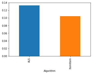
user_ndcg.groupby('Algorithm').nDCG.mean()

Algorithm
ALS         0.133029
ItemItem    0.104659
Name: nDCG, dtype: float64

user_ndcg.groupby('Algorithm').nDCG.mean().plot.bar()

<matplotlib.axes._subplots.AxesSubplot at 0x2643b7a0cf8>